- Đổi mới
- Bài viết về cách áp dụng PCI
- Giao dịch danh mục
Portfolio Optimization through PQM Method (Part 2)
Suppose that an investor is really ready to accept a higher risk level for increasing the expected return of the portfolio. Let the maximum acceptable standard deviation of the return of the portfolio be 2.5%. We will carry out the optimization procedure of weight coefficients for searching for the maximum return of the portfolio with an additional restriction on the standard deviation (it should not exceed 2.5%)
The solution leads us to the following composition of P3: MCD stocks again got the greatest weight (61.63%). Then DIS (21.74%), HON (14.17%), IBM (1.61%) and HD (0.84%) were ranged in weight descending order. KO stocks got zero weight and are not included in portfolio P3.
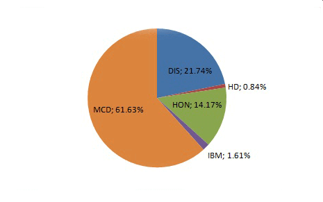
As a result, the portfolio P3, formed to maximize the expected return under the condition of not exceeding the standard deviation level of 2.55, gave the expected monthly return of 0.65% and the Sharpe ratio of 0.26.
Table 4: Realized returns, standard deviations and Sharpe ratios of P1, P2 and P3 portfolio
| P1 | Р2 | Р3 | |
| Mean Return | 0.49% | 0.24% | 0.40% |
| StDev | 4.25% | 5.73% | 4.51% |
| Sharpe Ratio | 0.11 | 0.04 | 0.09 |
Through PCI tools let us build a chart reflecting the dynamics of portfolio P3, including five assets with corresponding weights in the base part, and Dow Jones Industrial Average index in the quoted part.
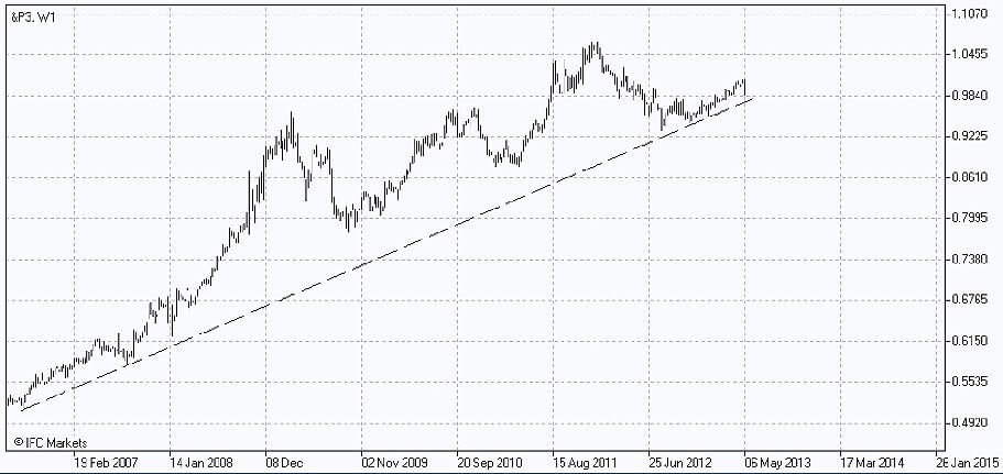
We can as before follow a growing structure. The growth during the whole observed period came to be more considerable than in case of P2, but the fluctuation during the crisis looks more significant – a direct result of the increase of the allowable risk.
To make the picture complete, let us also build a portfolio for an investor seeking to maximally get rid of risks by diversifying. To do that, we will resort to the optimization procedure of the weights of the available assets and to the search for the minimum value of the standard deviation. The portfolio P4 is characterized by the following set of weights:
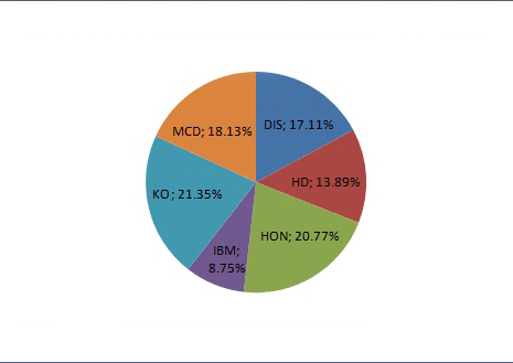
The diagram shows that this time the largest weight coefficient fell on KO stocks (21.35%), after all it was the asset for which we got the smallest standard deviation from input data. Then HON (20.77%), MCD (18.13%), DIS (17.11%), HD (13.89%) and IBM (8.75%) were ranged in descending weight order. That portfolio is characterized by expected return of 0.45%, standard deviation of 1.60% and the Sharpe ratio of 0.28.
Table 5: Realized returns, standard deviations and Sharpe ratios of P1, P2, P3 and P4 portfolios
| P1 | Р2 | Р3 | Р3 | |
| Mean Return | 0.46% | 0.52% | 0.65% | 0.45% |
| StDev | 1.74% | 1.72% | 2.50% | 1.60% |
| Sharpe Ratio | 0.26 | 0.30 | 0.26 | 0.28 |
PCI toolset will again help in building the chart of the portfolio and estimating its behavior in relation to Dow Jones Industrial Average index in the examined period of time.
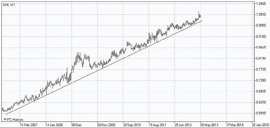
It is amazing how calm the behavior of portfolio P4 looks. Though the absolute growth during the whole period is lower than in case of previously formed portfolios, comparatively narrow range of fluctuations, reflecting lower volatility, has its advantages.
If we plot all four portfolios (Р1, Р2, Р3, Р4), in the coordinates of risk and return we can confirm only that portfolio P2 (maximum Sharpe ratio) is preferred to the “random” portfolio P1, since its position (in the higher left sector relative to P1) indicates higher return and lower standard deviation.
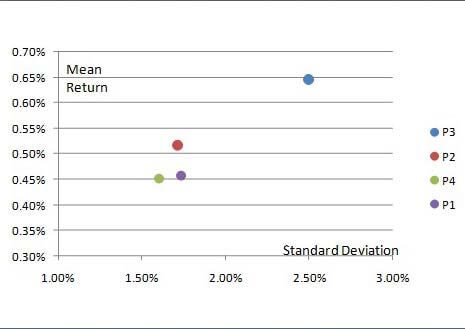
The choice between portfolios P2, P3 and P4 will depend on investor’s individual preferences and restrictions. If an investor is ready to accept relatively high risk level his choice will probably shift to portfolio P3 with the highest expected return (among the options considered). If an investor seeks to minimize risks, his choice may be portfolio P4, having the lowest standard deviation (among the options considered). We would call portfolio P2 a balanced portfolio, having the best return per unit of risk.
Charts, built through PQM method and PCI tools, visually confirm the opportunities of applying the principles of contemporary portfolio theory. Based on quantitative estimations of risk, return and covariance of various assets we have found a variety of “successful” portfolios, which have been systematically outperforming the market over recent years and meantime have met numerous investment preferences. Our analysis was based on only seven assets (6 stocks + index) of the same class of financial instruments. The potential gains from diversification can be considerably increased, if we add other asset classes into the analysis, which would have lower or negative correlation with each other. It is difficult even to imagine what kind of opportunities you will get in that case for applying PQM method for market analysis and trading.
See the beginning of the article "Portfolio Structure Optimization through PQM Method (part 1)"
Bài viết trước
- Định đề thứ tư của Dow trong chiến lược đầu tư
- Spread danh mục đầu tư trên cơ sở futures không thời hạn
- Danh mục Sharpe – “3 thủ lĩnh”
- Truy tìm danh mục "Tốt" và "Xấu" theo phương pháp Portfolio Quoting Method
- Hữu ích hóa danh mục đầu tư phương pháp PQM (phần 1)
- Stock Portfolio Construction | Stock Portfolio Analysis - Pportfolio Quoting Method PQM
