- Trading
- Program Trading
- Advisors for NetTradeX
- Creation of a neural network in NTL+
Creation of a neural network in NTL+
Introduction
Artificial neural networks - mathematical models and their software or hardware implementations that are built on the principle of organization and functioning of biological neural networks - networks of neural cells (neurons) of the brain.
Currently, neural networks are used widely enough in many tasks of recognition, classification, associative memory, determining patterns, forecasting etc.
In order to work with neural networks there are separate mathematical products and additional modules for major mathematical software packages that provide wide capabilities of constructing networks of different types and configurations.
We, on the other hand, will attempt to create our own neural network from scratch by means of the NTL+ language and try at once its object-oriented programming capabilities.
Choosing a task
In this article, let us verify a hypothesis that on the grounds of past bars it is possible to predict with certain probability the type of the following bar: rising or falling.
This task is related to classification ones. We also have extensive historical information on financial instruments at our disposal, which allows using this historical data to obtain desired(expert) output. Because of this, we will create a network based on multi-layer perceptron.
Now, let us try to create a network that predicts on the basis of closing prices of k bars, the type of the following bar. If its closing price is higher than the closing price of the previous bar, we assume the desired output to be 1 (the price rose). In other cases, let us assume that the desired output is 0 (the price did not change or fell).
Constructing the network
In general, a multi-layer perceptron has one input layer, one or several hidden layers and one output layer. Having a single hidden layer is enough for transforming inputs in such a way to linearly divide the input representation. Using more hidden layers often causes significant decrease in the training speed of a network without any noticeable advantage in learning quality.
Let us settle on a network with one input layer, one hidden and one output layer. The following figure shows the architecture of our network in general terms.
x1 - xn - inputs (closing prices), wi,j - weights of edges coming from i-node and going to j-node;
y1 - ym neurons of the hidden layer, o1 - ok outputs of the network.
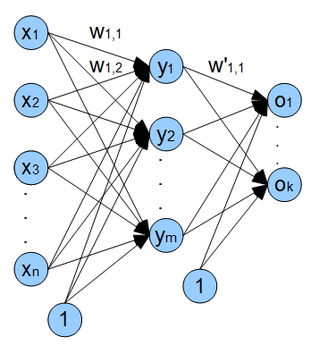
Additionally, there are bias inputs in the network. Usage of these inputs provides the capability of our network to shift activation function along the x-axis, thus not only can the network change the steepness of the activation function but provide its linear shift.
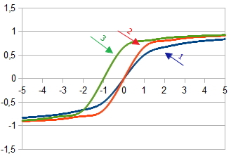
1. Graph of the activation function  at
at  = 1
= 1
2. Graph of the activation function  at
at  =2 and
  = 1
= 1
3. Graph of the activation function with the shift  at
at  =2,
=2,  = 1 and
  = 1
= 1
The value for each node of the network will be calculated according to the formula:
 , where f(x) - activation function, and n the number of nodes in previous layer.
Activation functions
Activation function calculates the output signal, received after passing the accumulator. Artificial neuron is usually represented as a non-linear function of a single argument. Most often the following activation functions are used.
Fermi function (exponential sigmoid):
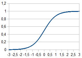
Rational sigmoid:

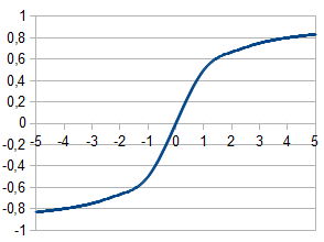
Hyperbolic tangent:
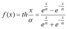
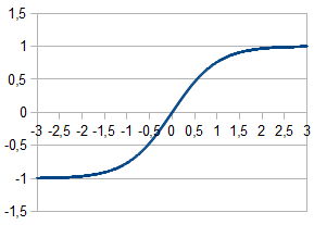
In order to compute outputs of each layer, rational sigmoid was chosen because its calculation takes less processor time.
Training process of the network
To train our network, we will implement the back propagation method. This method is an iterative algorithm that is used to minimize the error of work of a multi-layer perceptron. The fundamental idea of the algorithm: after calculating the outputs of the network, adjustments for each node  and error ω for each edge are calculated, at that the error calculation goes in the direction from network outputs to its inputs. Then the correction of weights ω takes place in accordance with the calculated error values. This algorithm imposes the only requirement on the activation function - it must be differentiated. Sigmoids and hyperbolic tangent comply with this requirement.
Now, to carry out the training process, we need the following sequence of steps:
- Initialize the weights of all edges with small random values
- Calculate adjustments for all outputs of the network
 , where oj - calculated output of the network, tj - expected(factual) value
 - For each node except for the last calculate an adjustment according to the formula
 , where ωj,k
weights on the edges coming from the node for which the adjustment is calculated and
 calculated adjustments for the nodes situated closer to the output layer.
- Calculate the adjustment for each edge of the network:
 , where oi calculated output of the node from which the edge comes. The error is calculated for this edge and
  - calculated adjustment for the node to which the specified edge comes.
 - Correct weight values for all edges:

- Repeat steps 2 - 5 for all training examples or until the set criterion of learning quality is met
Preparing input data
It is necessary to prepare input data to perform training process of the network, the input data of high quality have a significant impact on the work of the network and speed of stabilizing its coefficients ω, i.e. on the training process itself.
All input vectors are recommended to be normalized, so that their components lie in the range [0;1] or [-1;1]. Normalization makes all the input vectors commensurate in the training process of the network, therefore correct training procedure is achieved.
We will normalize our input vectors - transform the values of their components to the range [0;1], to do so let us apply the formula:

Closing prices of bars will be used as components of the vector. The ones with indices [n+k;n+1] will be fed as outputs, where k - input vector dimension. We will determine the desired value based on the n-th bar.
We will form the value on the grounds of the following logic: if closing price for the n-th bar is higher than the closing price of the n+1 bar (the price rose), we will set the desired output to 1, in case the price fell or did not change, we will set the value to 0;
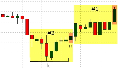
The bars involved in the formation of each set are highlighted in yellow in the figure, the bar that is used to determine the desired value is highlighted in orange.
The sequence of provided data also affects the training process. The training process happens steadier if all input vectors corresponding to 1 and 0 are fed evenly.
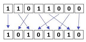
Additionally, let us form a separate set of data that is used for the assessment of effectiveness of our network. The network will not be trained on this data and it will only be used for calculating the error with the method of least squares. We will add 10% of initial examples to a test data set. As a result, we will use 90% of the examples for training and 10% for testing.
Function, calculating the error with the method of least squares, looks like this:
 ,
,
where  - output signal of the network and
  - desired value of the output signal.
Now let us examine the script code, preparing input vectors for our neural network.
Let us consider DataSet class - set of data. The class includes:
- Array of vectors of input values - input
- Formed output value - output
- 'Normalize' method - normalization of data
- 'OutputDefine' method - determining actual value on the relationship of prices
- 'AddData' method - recording values in the input vector array and actual value variable
- 'To_file' method - collecting data in the common array for the subsequent recording in the file
Now let us examine the program code, used in the Run() function and performing the following sequence of actions:
- Loading all historical data that is available in the terminal to an interior array. Loading is performed for the symbol and timeframe for which the current chart is displayed.
- Trimming the bar array to the size that is n-fold of the input vector + output value
- Forming the arrays of input vectors; normalizing these vectors; determining desired value 0 or 1
- Forming the array of sorted input vectors where the vectors corresponding to 0 and 1 alternate successively
- Recording the main part of the array with sorted input vectors in the file with data and recording the remaining part of data in the array for testing and, subsequently, estimating with the method of least squares.
You also need to declare the global variable int state = 0 in this file, the variable is required for alternation of input vectors.
Creating network classes
We will need for our network:
- an instance of 'layer' class for connecting input and hidden layers of the network
- an instance of 'layer' class for connecting hidden and output layers of the network
- an instance of 'net' class for connecting layers of our network
Creating the class 'layer'
Now, we will need the class, containing the following properties and methods:
- array 'input' for storing inputs of the network
- array 'output' for storing outputs of the network
- array 'delta' for storing adjustments
- two-dimensional array 'weights' for edges' weights
- method 'LoadInputs' for assigning the values specified in the input array to inputs of the layer
- method 'LoadWeights' for loading weight values of the layer from the hard drive
- method 'SaveWeights' for saving weight values of the layer to the hard drive
- constructor allocating the necessary memory volume for the used arrays
- method 'RandomizeWeights' - filling weights with random values
- method 'OutputCalculation' - calculating output values
- methods 'CalculatingDeltaLast' and 'CalculatingDeltaPrevious' - calculating adjustment values
- method 'WeightsCorrection' - correcting weight values
- additional (diagnostic) methods for displaying information on the screen:
- PrintInputs() - printing the inputs of a layer
- PrintOutputs() - printing the output of a layer (is called after calculating output by means of 'OutputCalculation')
- PrintDelta() - printing adjustments for a layer (should be called after calculating adjustments by means of 'CalculatingDeltaLast' or 'CalculatingDeltaPrevious')
- PrintWeights() - printing weights ω of the layer
- Method 'Calculate' - binding our layers for the calculation of the network output. This method will be used later for the work with the trained network
- Method 'CalculateAndLearn' - computing outputs, adjustments and errors. We will call the previous method to calculate outputs, and for adjustments and errors it will call corresponding methods of each layer
- Method 'SaveNetwork' - saving coefficients (weights) of the network.
- Method 'LoadNetwork' - loading coefficients (weights) of the network.
- creates object NT of the class 'net'
- reads coefficients(weights) ω and loads them in NT
- creates arrays of inputs and outputs of the network
- reads inputs in a loop and places them in 'x' array, reads outputs and places them in 'reals' array
- calculates the output of the network, feeding 'x' array as an input
- computes error as the sum of squares of differences between all calculated values and expected(factual) values
- when the end of file is reached, we display the error and terminate the work of the script
Let us remove the created class to a separate file. Besides, this file will also contain network configuration: number of nodes in input, hidden and output layers. These variables were placed outside the class in order for them to be used in the script for input data preparation.
We will also need additional functions that we will place outside the classes. These are 2 functions: normalization of an input vector and activation function.
Creating the class 'net'
We will need the class combining our layers into a joint network, therefore such a class should have:
Checking the work of the network
In this subsection, we will check the work of our network on an elementary example that will be used to determine the correctness of classification of input vectors.
To this end, we will use a network with two inputs, two nodes of the hidden layer and one output. We will set the parameter nu to 1. Input data will be represented as alternating sets with the following contents:
input 1,2 and expected value 1
input 2,1 and expected value 0
They will be specified in the file in this form:
Feeding different number of training sets to the input, we can observe how the training process of our network is advancing.
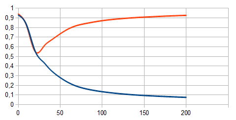
The red line on the graph shows the training sets corresponding to 1. The blue line - corresponding to 0. The number of training examples is laid off along the x-axis and the calculated network value - along the y-axis. It is obvious that when there are few bars (25 or fewer) the network does not recognize different input vectors, when there are more of them - the division into 2 classes is apparent.
Evaluation of the network functioning
In order to evaluate the effectiveness of training, let us use the function calculating the error with the method of least squares. To do so, let us create the utility with the following code and run it. We will need two files for its work: "test.txt" - data and desired values (outputs) that are used in error correction and "NT.txt" - the file with the calculated coefficients (weights) for the work of the network.
This script performs the following sequence of actions:
Creating an indicator
Let us create an indicator showing the decision of the network about the next bar by means of a histogram. The logic of work of the indicator is straightforward. Value 0 will correspond to the falling value of the next bar, value 1 - rising value, and 0.5 - the events of decreasing and increasing of closing price are equally possible. To show the indicator in a separate window, we will specify
#set_indicator_separate, it is also necessary to determine the file where the class 'net' is defined, we will include the file in the line #include "Libraries\NN.ntl". Moreover, we will need a variable for storing computed output of the network for the given input, if there is only one output value, then it is enough to have one variable, but the network can have several outputs, therefore, will need an array of values: we declare it in the line array . In the initialization function of our indicator we will specify indicator's parameters, its type, bind values of histogram with two buffers of values. We will also need to restore parameters of our network, i.e. load in it all weight coefficients, computed during training process. This is done by means of the method LoadNetwork(string s) of object NT, with the only parameter - file name, containing weight coefficients. In the function Draw we form input vector x corresponding to closing prices of the bars with indices [pos+inputVectorSize-1; pos], where 'pos' - number of the bar that we compute the value for and 'inputVectorSize' dimension of input vector. At the end, the method 'Calculate' of object NT is called. It returns an array of values (if our network have several outputs), but because we have only one output, we will use the element of the array with index 0.

The diagram above shows the network forecast of the subsequent bar. Values from 0.5 to 1 suggest the higher possibility that the subsequent bar will rise than fall. Values from 0 to 0.5 imply higher possibility of falling rather than rising. Value 0.5 suggests the state of ambivalence: the next bar might go up or down.
Summary
Neural networks are powerful tools for data analysis. This article covered the process of creation of a neural network by means of object-oriented programming in the NTL+ language. Usage of object-oriented programming allowed simplifying the code and made it much more reusable in the future scripts. In the presented implementation we needed to create the class layer defining a layer of the neural network and the class net defining the network in general. We used the class 'net' for the indicator, computing error and calculating network internal weights. Moreover, it was presented how to use the trained network by the example of the indicator-histogram that provided the network's forecast of the price change.
